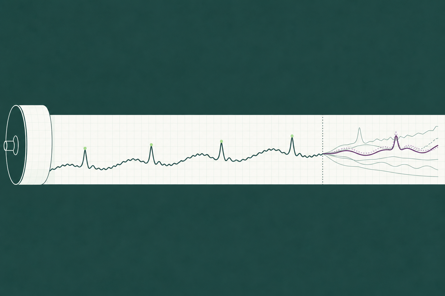
Time series forecasting is the practice of predicting future values of a measurement from its own past, using the patterns in the sequence (level, trend, seasonality and the relationship between one period and the next) to extend it forward. For demand, the series is units sold or shipped per week or month, and the forecast is the number the supply plan will be built on.
Demand series are harder than most. They carry promotions that the past does not announce, stockouts that record the units you had rather than the units people wanted, and new items with no past at all. So instead of describing the demand forecasting methods in the abstract, this post runs six of them on one SKU: 104 weeks of weekly demand with seasonality, a trend, a price change and ten promotions, scored on a 13-week hold-out with WMAPE. The result we want you to carry away is a specific one. The five classical methods landed between 18% and 22% WMAPE, and the machine learning model landed at 7%. Then we removed the promotion, price and holiday inputs from that same model and it scored 16%, in line with the classical pack, and on the weeks with no promotion the two versions tied at 5%. Model choice moved the error by a few points. Knowing the promotion calendar moved it by nine. The error is in the calendar, and the method that wins is the one that can read it.
What is time series forecasting?
A time series is any measurement taken at regular intervals: weekly unit sales, daily orders, monthly shipments. Time series forecasting assumes the sequence contains structure that will persist, and each method is a different bet on what that structure is. The naive method bets that nothing changes. Seasonal methods bet that last year repeats. Smoothing methods bet that recent history matters more than old history. ARIMA bets that the next value depends on the last few values and the last few errors. Machine learning methods can bet on all of those and on outside drivers at the same time.
What every classical method shares is a single input: the series itself. That is the strength of the family, since the data is always available, and it is the limit of the family, since anything that is not in the series cannot be forecast from it.
The four parts of a demand series: trend, seasonality, cycle, noise
Decompose a demand series and four components fall out.
Trend is the long-run direction: our SKU grows by roughly 10% a year as distribution widens. Seasonality is the repeating pattern within a year: our SKU peaks in late November and bottoms out in February, swinging about 22% either side of its average. Cycle is the slower, irregular wave driven by the economy or the category, which most weekly demand forecasting ignores because two years of data cannot see it. Noise is what is left, the week-to-week variation nothing explains, and on our SKU it runs at about 6%.
Promotions do not belong to any of the four. A promotion week sits 55% above the underlying level on our SKU, and the week after it sits 20% below, and neither the spike nor the dip repeats on a calendar the series can learn. The classical methods have to treat them as noise or as seasonality, and both choices fail in ways you can see below.

The dataset: 104 weeks of one SKU
We built the dataset rather than borrowing one, so the answer key is known. It behaves like a promoted consumer product: a base of about 1,000 units a week, a trend of roughly 10% a year, annual seasonality peaking in late November, a 55% uplift in promotion weeks followed by a 20% dip the week after, a 12% lift in holiday weeks, a shelf price increase from $24.99 to $25.99 after week 60, and 6% random noise. Ten promotions fall across the two years. The file has one row per week with the demand, a promotion flag, a post-promotion flag, a holiday flag and the shelf price.
Download the 104-week dataset and every method’s forecast (Excel). Weeks 1 to 91 are the training window; weeks 92 to 104 are the hold-out. Error and WMAPE columns are live formulas.
Every method is trained on weeks 1 to 91 and asked for a 13-week forecast of weeks 92 to 104, which is one planning quarter ahead with no refitting in between, the way a quarterly supply plan actually uses a forecast. The hold-out contains two promotions (weeks 96 and 102), two holiday weeks (92 and 101), and the start of the seasonal climb into the fourth quarter. We score each method with WMAPE, the sum of absolute errors divided by the sum of actual demand, because it weights each week by its volume, and our guide to measuring forecast accuracy explains why WMAPE is the practitioner’s default over MAPE. Alongside WMAPE we note the week each method missed by the most, because the worst week tells you what the method cannot see.
Method 1: naive and seasonal naive
The naive forecast assumes next week equals last week. Every week of the quarter is forecast at 975 units, the last training value. It cannot see the season, the trend or the promotions, and it scores 20.2% WMAPE. Its worst week is 102, a promotion week in the seasonal climb, where demand reached 2,062 against a forecast of 975. The naive forecast is still worth running, since any method that cannot beat it is adding nothing.
The seasonal naive forecast assumes this week equals the same week last year. It picks up the seasonal climb and scores 18.6%, better than the naive. Its failure is instructive: last year’s promotion fell in week 42, so the forecast for week 94 (52 weeks later) is 1,447, and demand came in at 986. This year’s promotion ran in week 96 instead, where the forecast was 964 against 1,474 actual. The method remembered the promotion and put it on the wrong date.
Method 2: moving average forecast
The moving average forecast assumes demand is the recent average plus noise. A four-week moving average of the last training weeks gives 947 units, held flat across the quarter. It is the smoothest line in the set and the worst score: 21.5% WMAPE, with the same worst week (102) as the naive. A moving average lags every turn by half its window, and a flat forecast into a rising season lags the whole quarter. It suits flat, noisy items where the goal is to filter the noise, and almost nothing else.
Method 3: exponential smoothing and Holt-Winters
Simple exponential smoothing assumes recent weeks matter more than older ones. It weights the history with exponentially decaying weights and produces a flat forecast of 961 units: 20.9% WMAPE, barely different from the moving average, for the same reason. The level it estimates is fine. A level is all it can produce.
Holt-Winters assumes a level, a trend and a seasonal pattern, each updated as data arrives. With a 52-week season and an additive damped trend, it is the strongest classical method on this SKU: 18.0% WMAPE, the best of the five. It follows the seasonal climb and the trend, and its forecast for the normal weeks is close. Its failure is the same as the seasonal naive’s, only smoother. Last year’s week-42 promotion was learned as part of the seasonal index, so Holt-Winters forecasts 1,525 units for week 94, against 986 actual, and then has nothing in the index for week 96, where the real promotion ran. Its worst week is still 102, at 1,193 forecast against 2,062 actual.
This is the pattern to recognize in your own planning system: a seasonal model that is excellent on the baseline and wrong by a promotion’s worth whenever the marketing calendar moves.

Method 4: ARIMA
ARIMA assumes the next value depends on recent values and recent errors, after differencing away trend and season. We fit a seasonal ARIMA with one seasonal difference (so the model works on the change from the same week last year) and one autoregressive and one moving average term. It scores 19.3% WMAPE, between the seasonal naive and Holt-Winters, and its worst weeks are the same two: the phantom promotion in week 94 (1,556 forecast against 986) and the real one in week 102. ARIMA is a serious method for stable series where the autocorrelation carries information, and it needs tuning per series, which is why it is rarely the default at SKU scale. On a promoted item with two years of history, it has the same blind spot as every other model in this section.
Method 5: machine learning with demand drivers
Machine learning with drivers assumes demand is a function of things you know in advance. We trained a gradient boosting model on the trend, the week of year, last year’s demand for the same week, and four driver columns: the promotion flag, the post-promotion flag, the holiday flag and the shelf price. It scores 7.0% WMAPE, less than half the error of the best classical method. It forecasts the week-96 promotion at 1,534 against 1,474 actual, and the post-promotion dip in week 97 at 808 against 788. Its worst week is week 102, where the second promotion combined with the holiday the week before and the seasonal climb, and the model forecast 1,570 against 2,062: right about the spike, short on its size, with only ten promotions in the history to learn from.
Then we ran the experiment that matters. Same algorithm, same settings, same training window, with the four driver columns removed. That version scores 16.1% WMAPE, inside the classical pack. On the seven hold-out weeks with no promotion or post-promotion effect, the two versions are tied, at 4.9% and 5.0%. All of the gap between 16.1% and 7.0% is promotion weeks. The algorithm did not win this comparison. The inputs did.
That result generalizes. Our work on demand drivers comes to the same place from the other direction: most of a forecast’s accuracy comes from a small number of inputs that actually move demand, and in the Accuracy Report, one consumer hardware company went from 20 variables to 4 and improved its forecast by doing so. The hard part of machine learning forecasting is rarely the model. It is knowing which four columns to feed it, and having them clean and available for the weeks you are forecasting.
One note on foundation models. Pretrained time series models such as Amazon’s Chronos and Google’s TimesFM take a series with no training and return a forecast, and they do well on the baseline pattern. In their basic form they see only the series, so they share the classical blind spot on promotions unless drivers are added through a covariate mechanism. A dedicated post on them is in the pipeline.

Results: all six methods on one table
| Method | What it assumes | Hold-out WMAPE | Best for | Breaks when |
| Naive | Next week equals last week | 20.2% | Very short horizons on stable items; the baseline every other method must beat | Anything changes: season, trend, promotion |
| Seasonal naive | This week equals the same week last year | 18.6% | A quick seasonal baseline | Promotions move dates; the level shifts year over year |
| Moving average (4-week) | Demand is the recent average plus noise | 21.5% | Flat, noisy items | Trend or seasonality; the average lags every turn |
| Holt-Winters | Level, trend and a repeating seasonal pattern | 18.0% | Seasonal items with two or more years of clean history | Last year’s promotions are baked into the seasonal index |
| ARIMA (seasonal) | The next value depends on recent values and errors, after differencing | 19.3% | Stable series where autocorrelation carries signal | Short history; one-off events; needs tuning per series |
| ML with drivers (gradient boosting) | Demand is a function of known drivers: promotions, price, holidays, season, trend | 7.0% | Promoted, priced and seasonal items where the drivers are known in advance | Drivers are missing or wrong; structural breaks with no history |
Two reference rows from the same run: simple exponential smoothing scored 20.9%, and the gradient boosting model without drivers scored 16.1%.
This pattern is the one the Accuracy Report measured at scale. In 15 head-to-head deployments, an AI forecast beat the incumbent statistical forecast in every case reviewed, with error reductions from 14% to 56%. The incumbents in those deployments were the methods in the top five rows of this table, or planners adjusting them, and the mechanism was the one in Method 5: more of what moves demand reaching the model.

Where time series forecasting breaks
Four situations defeat every method in the table, including the last one, and each has its own fix.
New products. No history means no series. The early forecast has to come from analogues (how similar launches behaved), from drivers (distribution, price, marketing plan) and from judgment, until the item has enough weeks to stand on its own. Our guide to forecasting new products walks through that sequence.
Intermittent demand. A series that is zero most weeks and large occasionally has no level, trend or season to extend. Smoothing it produces a small positive number every week that is wrong every week. Intermittent-demand methods such as Croston’s separate the question of when demand arrives from how much arrives, and driver signals (which customers are due to order) often do better than either.
Structural breaks. A new competitor, a lost distribution channel, a reformulation. The history before the break describes a product that no longer exists, and every method trained on it will forecast the old product. The fix is to detect the break early, which is a monitoring problem, and to shorten the history or add a feature that marks the change.
Stockout-censored history. A week where the shelf emptied on Wednesday records three days of demand as seven. Every method then learns that demand is lower than it was, and forecasts low into the next stockout. Flag the stockout weeks and replace recorded sales with an estimate of demand before training anything.
How to choose a time series forecasting model
Our decision path is short, and it starts with the data rather than the method.
Less than a year of history: you cannot estimate seasonality, so use a seasonal analogue from a similar item, or a driver-based model with the season borrowed from the category. Holt-Winters and seasonal ARIMA are out until the second year.
One to two years, no promotions or price changes: Holt-Winters is the sensible default and is hard to beat on a clean seasonal series. Run the seasonal naive next to it as the check.
Promotions, price moves or holidays that matter: the driver columns decide the result, as Method 5 showed. Use a model that accepts them, and spend the effort on getting the promotion calendar into the data for future weeks, not on tuning the algorithm.
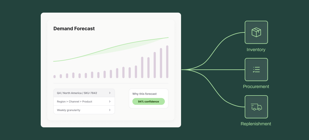
Thousands of SKUs: the honest answer is that the right method differs by item and changes over time, and no planning team can hand-select per SKU. This is the problem DemandForecast.ai is built for. The platform runs an ensemble of models per SKU, selects and reweights them as new data arrives, feeds them the drivers (promotions, pricing, seasonality, external signals) that this post shows matter most, and explains which drivers moved each forecast so a planner can check the reasoning rather than the arithmetic. The deployments in the Accuracy Report produced their first forecast in under four weeks, on portfolios from a few hundred SKUs to more than 100,000, which is the scale at which method selection stops being a spreadsheet exercise.

Everything here is yours to download and rerun, and the fastest way to test the argument is to add your own promotion calendar to your own history and see what happens to the worst week. If you would rather see it run on your SKUs with the drivers already wired in, request a demo.