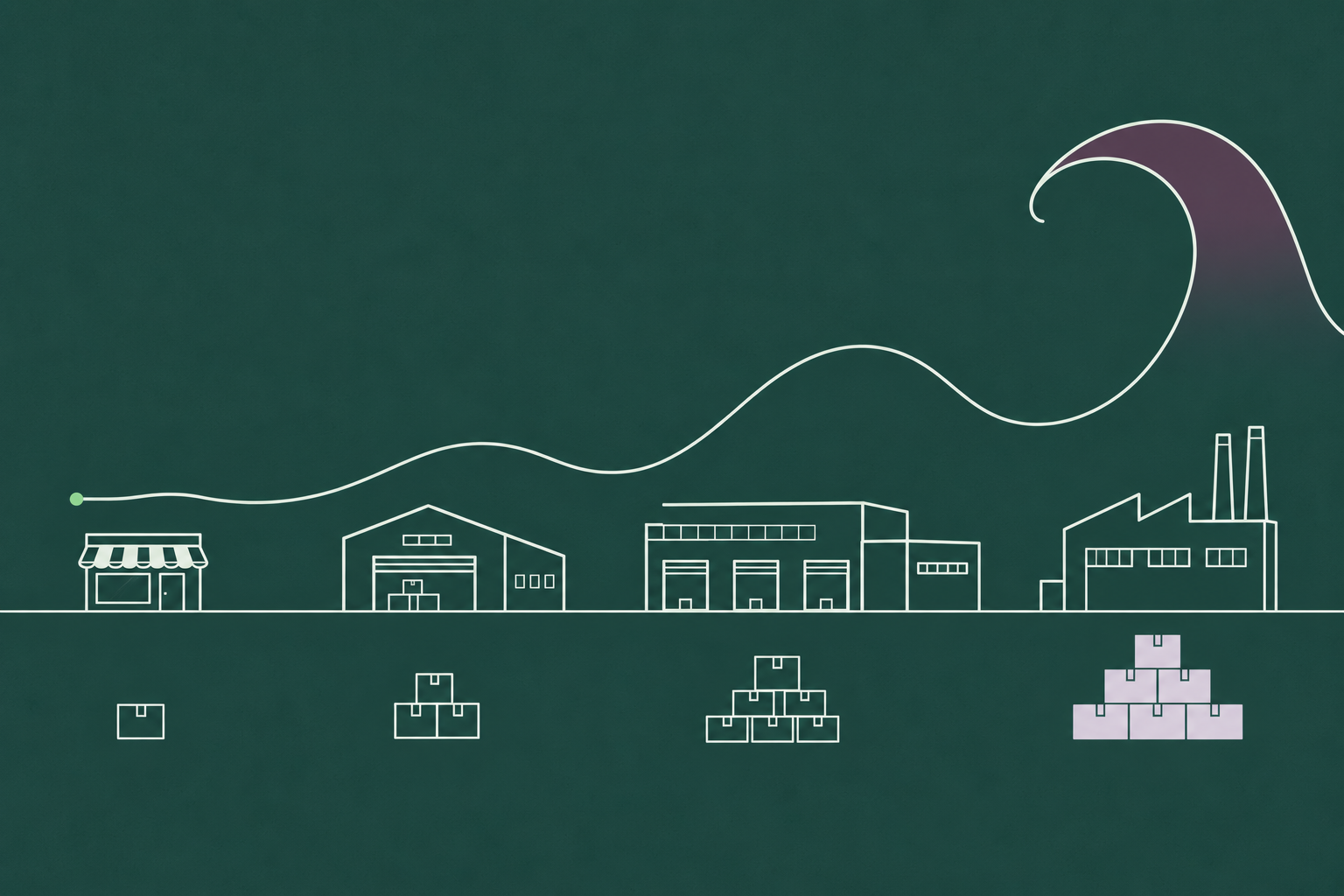
The bullwhip effect is the amplification of demand variability as orders move upstream through a supply chain: a small change in what consumers buy becomes a larger swing in retailer orders, a larger swing again at the distributor, and the largest swing of all at the factory. The name describes the shape. A flick at the handle produces a wide crack at the tip.
Most explanations list four causes and move on. We wanted to show the whip forming, so this post builds one in a table you can follow week by week: consumer demand rises from 100 units to 110 and stays there, and four tiers that each forecast from the orders they receive turn that 10-unit step into a 160-unit swing at the factory, followed by two weeks of zero production. Then we run the same chain with one change, every tier forecasting from end demand, and the whip loses its handle. Of the four classic causes, demand signal processing is the one a forecast fixes, which is why the forecast is where we would start.
Why planners care: the factory in that table builds for demand that never existed, and the cost of excess inventory it creates lands downstream as markdowns, write-offs and warehouse space months after the shelf absorbed the original 10-unit change.
What is the bullwhip effect?
Each company in a supply chain sees only the orders placed by its immediate customer, and plans from them. When a retailer sees demand tick up, it orders a little more than the increase to rebuild its buffer. The wholesaler sees that larger order, reads it as rising demand, and orders more still. Every tier repeats the logic on an already amplified signal, so the swing compounds. When demand ticks back down, the same logic runs in reverse and the factory sees orders collapse.
Jay Forrester described the dynamics in 1961 in Industrial Dynamics, simulating how order delays and feedback in a distribution chain produce oscillations far larger than the consumer change that started them. The name came later. Hau Lee, V. Padmanabhan and Seungjin Whang wrote “The Bullwhip Effect in Supply Chains” in the Sloan Management Review in 1997, after Procter and Gamble executives used the term to describe what they saw in Pampers orders. That paper named the four causes most people still cite.
How the bullwhip effect builds: a four-tier example
Our rules are deliberately simple, and they are the rules many planning systems still run.
- Consumer demand runs at 100 units a week, steps up to 110 in week 3 and stays there.
- Four tiers sit above the consumer: retailer, wholesaler, distributor, manufacturer. Each one sees only the orders from the tier below it.
- Each tier forecasts next week’s demand as the average of the last two weeks of orders it received.
- Each tier holds a target stock of two weeks of forecast and orders enough to ship this week’s demand and restore that target. Orders cannot go below zero.
- Replenishment is immediate, to keep the arithmetic readable. Real lead times make every number below worse.
Here is what each tier orders, week by week.
| Week | 1 | 2 | 3 | 4 | 5 | 6 | 7 | 8 |
| Consumer demand | 100 | 100 | 110 | 110 | 110 | 110 | 110 | 110 |
| Retailer orders | 100 | 100 | 120 | 120 | 110 | 110 | 110 | 110 |
| Wholesaler orders | 100 | 100 | 140 | 140 | 100 | 100 | 110 | 110 |
| Distributor orders | 100 | 100 | 180 | 180 | 60 | 60 | 120 | 120 |
| Manufacturer production | 100 | 100 | 260 | 260 | 0 | 0 | 60 | 180 |
Follow one tier to see the mechanism. In week 3 the retailer sells 110, forecasts 105 (the average of 100 and 110), raises its stock target from 200 to 210, and orders 120: the 110 it sold plus 10 to rebuild the buffer. The wholesaler now sees 120 where it used to see 100, forecasts 110, lifts its target by 20, and orders 140. The distributor sees 140 and orders 180. The manufacturer sees 180 and schedules 260.
A 10% rise at the shelf has become a 160% rise at the factory, and the damage is only half done. In week 5 the retailer’s forecast catches up with the new level and its orders drop back to 110. The wholesaler sees orders fall from 140 to 110, cuts its target, and orders 100. The distributor sees a fall from 140 to 100 and orders 60. The manufacturer, sitting on the stock it built in weeks 3 and 4, sees orders fall from 180 to 60 and produces nothing for two weeks. By week 8 the factory has swung between 0 and 260 to serve a consumer who bought a steady 110 every week since week 3.

The four causes of the bullwhip effect
Lee, Padmanabhan and Whang grouped the causes into four, and each one shows up in a planning team in a recognizable way.
1. Demand signal processing. Every tier treats the orders it receives as a demand signal and updates its forecast from them. Because those orders already contain the tier below’s buffer adjustments, the forecast chases noise. In the table above this is the only cause at work, and it produces the whole whip on its own. In a planning team it looks like a weekly forecast review that moves the number every time a large customer order lands, with safety stock rebuilt on every forecast change, so each revision carries an order change with it.
2. Order batching. Companies accumulate demand and order in batches to spread fixed order costs, fill a truck, or hit a supplier minimum. The upstream tier then sees a lumpy stream of large orders separated by nothing, even when consumption is smooth. Picture a planning calendar that releases purchase orders on the last Friday of the month, and a supplier whose demand chart has four spikes a year labelled “quarter end”.
3. Price fluctuation and forward buying. Trade promotions, volume discounts and periodic price cuts invite customers to buy ahead. Orders spike during the deal and vanish afterwards, so the upstream tier sees the pricing calendar rather than consumption. The symptom is a promotion uplift followed by a trough the forecast never models, and a manufacturer staffing a line for a peak borrowed from next month.
4. Rationing and shortage gaming. When supply is short and the supplier allocates in proportion to orders, customers inflate their orders to secure a larger share, then cancel once supply recovers. The supplier reads the inflated orders as real demand and expands capacity for it. Think of the allocation spreadsheets of 2021 and the cancellation emails of 2022.
Three of these causes live in commercial policy and logistics. One lives inside the forecasting process itself. That distinction matters for where you start, and we come back to it below.

Real-world examples of the bullwhip effect
Procter and Gamble, Pampers. The example that named the effect. P&G’s logistics executives noticed that retail sales of diapers fluctuated, but not by much, since babies consume them at a steady rate. Distributor orders to P&G showed “a greater degree of variability,” and P&G’s own orders to suppliers such as 3M swung “even greater,” according to Lee, Padmanabhan and Whang’s 1997 account. The product with the most predictable end demand in the store had one of the least predictable order streams at the top of its chain.
Hewlett-Packard printers. In the same paper, HP’s reseller sales showed “some fluctuations over time,” reseller orders to the printer division showed “much bigger swings,” and the printer division’s orders to HP’s integrated circuit division showed “even greater fluctuations.” The chip plant, three tiers from the customer, planned around the wildest signal in the chain.
Consumer goods and chips, 2020 to 2022. The pandemic ran the whip at national scale. Demand for home goods jumped in 2020, retailers and suppliers ordered into stockouts and long lead times, and by spring 2022 the orders arrived into a market that had moved on. In the quarter ending April 2022, Target’s inventory was up 43% year on year on sales growth of 4%, and Walmart’s inventory was up 32% on sales growth of 2%, according to figures reported by AJ Bell. The markdowns that followed were the whip arriving at the retail tier. Semiconductors ran the same cycle with longer lead times: double ordering during the 2021 shortage pushed the industry to expand output by roughly a third between 2019 and 2022, and by early 2023 inventories sat about a quarter above healthy levels, as TechInsights’ Dan Hutcheson argued in asking whether the macro shortage had been real at all.

The beer game: the bullwhip effect in a classroom
Developed at MIT’s Sloan School in the early 1960s on Forrester’s work, the beer game is a tabletop simulation with four players: retailer, wholesaler, distributor and brewery. Each sees only the orders from the player downstream, and orders take two rounds to arrive. Consumer demand is a fixed script that steps up once and never moves again. Within a dozen rounds the brewery is swinging between huge production runs and nothing, and the players, who know nothing about the script, are convinced the end customer is erratic.
Sixty years on, it still works as a teaching tool because it removes every excuse: no bad data, no promotion, no shortage gaming, no incompetent player. Only the structure, and the structure is enough. Players learn in an afternoon that the oscillation is a property of the chain rather than of the people in it, which is the right frame for any planning team trying to fix it.
How to measure it: the bullwhip ratio
Planners measure the effect with a variance ratio.
Bullwhip ratio = variance of orders placed ÷ variance of demand received
A ratio of 1 means a tier passes variability through unchanged. Above 1, the tier amplifies. Below 1, it dampens, which is what a well-run tier with stable ordering rules should do. You can compute the ratio tier by tier, using each tier’s incoming demand as the denominator, or against end-consumer demand for every tier, which shows how far the whip has travelled.
Against consumer demand, the eight weeks in our example come out like this.
| Tier | Order swing (peak minus trough) | Bullwhip ratio versus consumer demand |
| Consumer | 10 units | 1.0 |
| Retailer | 20 units | 2.7 |
| Wholesaler | 40 units | 14.3 |
| Distributor | 120 units | 100 |
| Manufacturer | 260 units | 507 |
Those ratios grow so fast because consumer variance is tiny (one 10-unit step) while factory variance is enormous. Real chains rarely look that extreme, but the shape is universal: the ratio climbs with every tier added. To track your own, compute the variance of your purchase orders and the variance of your sell-through over the same weeks. The error metrics in our guide to measuring forecast accuracy tell you how good the forecast is; the bullwhip ratio tells you how much variability your ordering policy adds on top of it.

How to reduce the bullwhip effect
Remedies map onto the causes, and most of them give every tier the same picture of demand.
Share point-of-sale and sell-through data upstream. When the distributor and the manufacturer can see what consumers bought this week, they stop inferring it from the retailer’s orders. Demand sensing is the formal version: POS, channel inventory and order signals adjust the near-term forecast, so upstream tiers react to consumption rather than to a buffer rebuild two tiers down.
Order smaller and more often. Batching is a cost decision, so attack the cost. Electronic ordering, mixed-SKU truckloads and third-party consolidation lower the fixed cost per order and let the batch shrink. Vendor-managed inventory removes the retailer’s order decision entirely.
Stabilize prices. Every-day low pricing removes the reason to forward buy. Where promotions are essential, plan them with suppliers in advance so the uplift and the trough both appear in the forecast.
Allocate on history, not on orders. During shortages, allocating in proportion to past sales rather than current orders removes the incentive to inflate. Firm order commitments with cancellation penalties do the same.
Shorten lead times. Lead time multiplies the whip: every tier’s safety stock scales with it and every forecast error compounds over it. Faster replenishment shrinks both the buffer rebuild and the overcorrection.
Plan across tiers. A single S&OP process that reconciles demand, supply and inventory on one calendar stops each function from reacting to the others’ adjustments. The point of the monthly cycle is one agreed number, and one agreed number is the opposite of a whip.
Why the forecast is the first place to fix it
Every remedy above takes time, money or a negotiation with another company. The forecast is the one lever that sits entirely inside your own planning team, and it produced the whole whip in our example. So we ran the example again with a single change: every tier forecasts from consumer demand rather than from the orders arriving from the tier below. Buffers and ordering rules stay exactly as they were.
| Week | 1 | 2 | 3 | 4 | 5 | 6 | 7 | 8 |
| Consumer demand | 100 | 100 | 110 | 110 | 110 | 110 | 110 | 110 |
| Retailer orders | 100 | 100 | 120 | 120 | 110 | 110 | 110 | 110 |
| Wholesaler orders | 100 | 100 | 130 | 130 | 110 | 110 | 110 | 110 |
| Distributor orders | 100 | 100 | 140 | 140 | 110 | 110 | 110 | 110 |
| Manufacturer production | 100 | 100 | 150 | 150 | 110 | 110 | 110 | 110 |
Factory peak: 150 instead of 260. The two weeks at zero disappear. Each tier still adds its own buffer rebuild, so the peak grows by 10 units per tier rather than compounding, and every tier settles at 110 in the same week. It is still a chain with four buffers in it. It has lost its handle, because no tier is forecasting from another tier’s reaction.
DemandForecast.ai is built around that mechanism. The platform forecasts each SKU from end demand and the drivers that move it, such as promotions, pricing and seasonality, so the forecast reflects consumption rather than the order stream, and it explains which drivers changed so planners can see a buffer rebuild for what it is. Fewer forecasts then need a manual touch, which matters because manual overrides are how a planning team adds its own tier to the whip, reacting to the last large order by moving the number. In the Accuracy Report’s 15 head-to-head deployments, AI forecasts beat the incumbent forecast in every case reviewed, and the reduction in forecast error ran from 14% to 56%. A forecast that misses by less overreacts by less, and the deployments that improved it also reported overstock cut by up to 50%, which is the tip of the whip getting shorter.

If your factory’s order chart looks nothing like your customers’ sales chart, the gap between the two is the whip, and the forecast is where we would start closing it. Request a demo and we will show you what a forecast built from end demand looks like on your own SKUs.