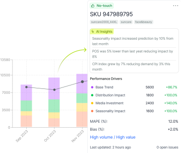
Safety stock is the price a business pays for forecast error.
That framing changes how you should read every formula on this page. The largest variable in the statistical safety stock calculation, the standard deviation of demand, is in practice a measurement of how far actual demand strays from what you planned for. Companies treat it as a fixed law of nature and buffer against it with inventory. It moves. And when it moves down, safety stock falls with it, at the same service level, with no risk added.
We’ll get to that lever. First, the formulas, all six of them, computed on one identical example so the differences between methods are visible instead of hidden behind six different sets of sample numbers.
The basic formula, up front: Safety stock = (maximum daily sales × maximum lead time) − (average daily sales × average lead time). With average daily sales of 100 units, a maximum of 120, an average lead time of 7 days and a maximum of 10, that’s (120 × 10) − (100 × 7) = 500 units.
What is safety stock?
Safety stock is extra inventory held beyond expected demand to protect against variability in demand and supply during the replenishment lead time. It functions as a buffer: when demand runs higher than forecast, or a supplier delivers late, safety stock covers the gap so service levels hold. It sits on top of cycle stock, the inventory that covers expected demand between orders.
The basic safety stock formula
Safety stock = (max daily sales × max lead time) − (average daily sales × average lead time)
The worked example used throughout this article:
- Average daily sales: 100 units
- Maximum daily sales: 120 units
- Average lead time: 7 days
- Maximum lead time: 10 days
- Target service level: 95%
- Standard deviation of daily demand: 15 units
- Standard deviation of lead time: 1.5 days
Basic method: (120 × 10) − (100 × 7) = 1,200 − 700 = 500 units.
The appeal is simplicity: four inputs, no statistics. The weakness is that it plans for maximum demand and maximum lead time occurring simultaneously, an event far rarer than either alone. It systematically overbuys protection, and it says nothing about what service level 500 units actually delivers.
Safety stock calculation: step by step
For the statistical method most planners should default to, the safety stock calculation runs as follows:
- Choose a service level. This is the probability of not stocking out during a replenishment cycle. 95% is a common starting point for A items.
- Convert the service level to a Z-score. For 95%, Z = 1.65. (Full table below. In Excel: =NORM.S.INV(0.95).)
- Measure the standard deviation of daily demand. Compute it from daily sales history over a representative period. In Excel: =STDEV.S(range). In our example, 15 units.
- Measure average lead time in days. Here, 7 days.
- Multiply: Safety stock = Z × standard deviation of demand × √(lead time) = 1.65 × 15 × √7 = 1.65 × 15 × 2.65 ≈ 65 units.
- Sense-check against history. Overlay the result on past demand spikes and confirm it would have covered the misses you care about.
Note the gap already: the basic method said 500 units, the statistical method says 65. Same product, same numbers. That spread is the subject of the next section.
6 safety stock formulas compared
All six methods below use the identical inputs from the worked example.
| # | Method | Formula | Result | Best suited for |
| 1 | Basic (max minus average) | (max daily × max LT) − (avg daily × avg LT) | 500 units | Quick estimates with no statistics available |
| 2 | Percent of cycle stock | 15% × (avg daily × avg LT) | 105 units | Rough portfolio-wide policy; ASCM guidance runs 10% to 20% |
| 3 | Days of supply | Chosen cover days × avg daily (3 days here) | 300 units | Simple operational rules; easy to explain, arbitrary in practice |
| 4 | Demand variability (statistical) | Z × σ demand × √(avg LT) | 65 units | Variable demand, reliable lead times |
| 5 | Lead time variability | Z × avg daily demand × σ lead time | 248 units | Stable demand, unreliable suppliers |
| 6 | Combined variability | Z × √(avg LT × σ demand² + avg demand² × σ lead time²) | 256 units | Both demand and supply are variable; the most complete method |
Six defensible methods, answers ranging from 65 to 500 units on identical inputs, a spread of nearly 8x. Multiply that spread across ten thousand SKUs and it’s the difference between a lean network and a warehouse expansion. Method choice deserves the same scrutiny as the inputs.
Method 6 is the technically correct default when both demand and lead time vary, and in the example it lands at 256 units. Notice why: with a lead time standard deviation of 1.5 days on 100 units of daily demand, supply variability contributes far more variance than demand variability does. The formula makes visible where your risk actually comes from, which is information the simpler methods throw away.
A short selection guide for the rest. Methods 1 through 3 belong in triage situations: no demand history, no statistical capability, or a need to set a provisional policy across thousands of SKUs in a week. They are heuristics, and their common failure is that nobody returns to replace them once the data exists. Method 4 fits businesses with dependable suppliers and noisy demand, which describes much of consumer retail. Method 5 fits the reverse, stable consumption with erratic replenishment, common in import-heavy and single-source supply bases. When you cannot say confidently which side dominates, that uncertainty is itself the argument for method 6, since it prices both.
One further discipline applies to all six: whatever method you choose, apply it consistently within a segment and document the choice. Mixed methods across comparable SKUs produce buffer differences that look like analysis and are actually accidents of spreadsheet history.
The Z-score table: service levels explained
The Z-score converts a target service level into the number of standard deviations of protection required. Because the normal curve flattens in the tail, each additional point of service costs progressively more inventory.
| Service level | Z-score |
| 90% | 1.28 |
| 95% | 1.65 |
| 98% | 2.05 |
| 99% | 2.33 |
Moving from 95% to 99% raises Z from 1.65 to 2.33, a 41% increase in safety stock for four points of service. This is why blanket 99% targets across a portfolio are an expensive habit, and why segmenting service levels by item value and criticality is standard practice in mature operations.
The hidden variable: forecast error
Every statistical method above contains σ demand, the standard deviation of demand. Guides treat it as a property of the market. Measured properly, against your forecast rather than against a simple average, it’s your forecast error, in units. Demand that’s genuinely volatile but well predicted requires little buffer; demand that’s stable but badly predicted requires a large one. The buffer protects against surprise, and surprise is a function of forecast quality.
That makes forecast accuracy a direct inventory lever, and the math is linear. In method 4, cut the demand standard deviation by 30% (from 15 units to 10.5) and safety stock falls from 65 units to 46, the same 30%, at an unchanged 95% service level. No service was traded away. The protection simply became unnecessary because the forecast got better.
Two honest caveats. In the combined formula (method 6), the same 30% improvement moves safety stock only from 256 to 252 units, because lead time variability dominates the variance in this example; forecast improvement pays off in proportion to how much of your variance is demand-driven. And realizing the reduction requires actually recalculating parameters after accuracy improves, which many organizations forget to do, leaving the old buffers frozen in the ERP. A grounding in demand forecasting practice helps in diagnosing which side of that split your network sits on.
The scale of improvement available is not hypothetical. Kenvue reduced forecast error (MAPE) by 37% by pairing its planners with AI-generated baseline forecasts. Error reduction of that magnitude, flowed through the safety stock formula on demand-variance-dominated SKUs, converts directly into working capital. The timeline can be short as well: one electrical components distributor forecasting more than 7,500 stocked SKUs reached 75% revenue-weighted forecast accuracy within 30 days of starting, fast enough that its next quarterly safety stock review ran on materially better error inputs.
When the formula breaks
Statistical safety stock assumes demand history predicts demand future, normally distributed around a stable mean. Three situations violate that assumption:
- New products. No history means no standard deviation to measure. Use analog items, plan for fast review cycles, and treat early buffers as provisional.
- Promotions. A promotion is a known, planned demand shift. Buffering it with safety stock treats signal as noise; forecast it explicitly instead, and keep promotional periods out of your baseline variance calculation.
- Supply shocks and trend breaks. A supplier failure or a step-change in demand invalidates the measured distributions. Formulas calibrated on the old world will confidently give you wrong answers in the new one; recalculate on post-break data as soon as enough of it exists.
In each case the failure is in the inputs rather than the algebra. The formula is only ever as good as the demand model feeding it.
Cutting safety stock without cutting service
The sequence most inventory reduction programs follow is to squeeze the buffers and hope service holds. The sequence that works runs the other way: improve the forecast, watch measured demand variability fall, then recalculate the buffers the formula now says you no longer need.
DemandForecast.ai is built for the first step. AI-generated baseline forecasts reduce the error that safety stock exists to absorb, and the platform tracks the accuracy metrics (MAPE, WMAPE, bias) that tell you when your buffer parameters are stale. The evidence for the approach is covered in our review of AI/ML forecasting, and our comparison of supply chain forecasting tools covers the wider software category. To see what your own demand variability looks like with a stronger baseline underneath it, request a demo.