Retail demand forecasting is the practice of predicting how many units of each product will sell, in each store or channel, over each day or week, so that buying, replenishment, allocation and staffing can be planned ahead of the sale. It differs from forecasting in most other industries in one way that decides everything else: the forecast is needed at the finest level of the business, where a single store sells a handful of units of a given item in a week, or none.
So we would argue retail forecasting is a granularity problem before it is a methods problem. The methods are the same ones used everywhere. What the guides skip is what happens to a method when the series underneath it gets thin. We built one SKU, twelve stores and eight weeks, and forecast it with one moving average at three levels: 11.8% weighted error at chain level, 17.8% at distribution center level, 38.2% at store level. A forecast that knew each store’s true average demand would still have scored 34% at store level. Most of the store-level error is noise no method removes, and knowing that changes what you forecast, where you reconcile, and what you hold a store forecast accountable for.
What is retail demand forecasting?
A retail forecast answers a four-part question: how many units, of which SKU, at which location or channel, in which period. The period is usually a week for replenishment and a day for fresh categories, labor scheduling and promotions. The location is a store, a dark store, a fulfillment center or an online channel, and the SKU is often a size-color variant, with its own series and its own zeros.
Four decisions run on the forecast. Replenishment uses it to set this week’s order for each store or DC. Allocation uses it to split a fixed buy across stores. Buying uses it months ahead to commit volume with suppliers, usually at chain or category level, and staffing uses it to put people on the floor when the units arrive. Each decision wants the forecast at a different level and horizon, which is the first sign that a retailer has a hierarchy of forecasts, never just one.
Why retail is harder to forecast than other industries
Five properties of retail demand make it harder than forecasting a manufacturer’s weekly shipments, even though the arithmetic is identical.
The number of series. A mid-sized chain with 20,000 SKUs and 500 stores has 10 million SKU-store combinations. The Walmart dataset behind the M5 forecasting competition covered 3,049 products in 10 stores, which produced 42,840 series across 12 levels of aggregation, most of them sporadic with many zeros. Nobody tunes 10 million models by hand, so whatever method you choose has to run unattended.
Sparse demand at the bottom. At store level most items sell a few units a week or none. A series of 0, 2, 0, 1, 3 has no trend or seasonality to extract, only a probability of selling and a size when it does.
Price and promotion are the biggest drivers. In most industries demand moves with the season and the economy. In retail it moves with the promotion calendar, the price ladder and the shelf position, all three decided inside the business and therefore available to the model in advance.
Short lifecycles. Fashion, seasonal and private-label items can be born and dead inside 26 weeks. Half the catalog has no history long enough to learn a season from.
Sales history records what was in stock. When the shelf is empty, the till records zero. The data carries last season’s stockouts as low demand, and a model trained on it will forecast low into the next one.
Same SKU, three levels: chain, DC and store
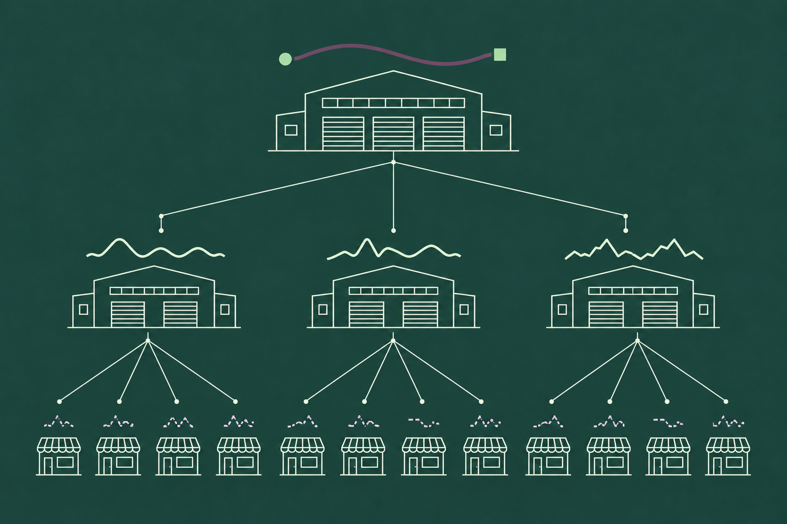
Our example is one SKU sold in 12 stores, served by three distribution centers of four stores each, over eight weeks. Store demand is Poisson around a mean that runs from 11 units a week at the busiest store to 0.6 at the quietest, with a chain-wide lift of 8% in weeks five to eight. Of the 96 store-weeks, 11 are zero and 35 are two units or fewer. The chain sells about 56 units a week.
Weeks five to eight are forecast with the same method at every level, a four-week moving average one week ahead, with no seasonality and no drivers, and scored with WMAPE: the sum of absolute errors divided by the sum of actual units.
| Level | Series | Average units per series per week | WMAPE, weeks 5 to 8 | WMAPE floor if the true average were known |
| Chain | 1 | 56 | 11.8% | 6.8% |
| Distribution center | 3 | 19 | 17.8% | 13.0% |
| Store | 12 | 4.7 | 38.2% | 34.1% |
Same SKU, same weeks, same method, and the error more than triples between the top of the hierarchy and the bottom. The last column is the one to study. Because we built the data, we know the true mean of every store and can score a forecast that is exactly that mean. It still misses by 34% at store level. Random variation around two or three units a week makes up most of the error, and no model fixes it, because it was never a modeling error.
Even within a level the gradient shows: the busiest distribution center scored 17.9%, and the quietest, with its four stores selling five units a week between them, scored 31.0%.
Two things follow. First, forecast where the data is dense and reconcile down. A chain or DC forecast can carry the season, the trend and the promotion, because it has enough units to show them. Hierarchical forecasting, which Hyndman and Athanasopoulos cover in their chapter on hierarchical and grouped time series, produces forecasts that add up across the whole structure, each level informed by the others. Second, where a store-SKU series is mostly zeros, use intermittent demand methods like Croston’s, which forecast the interval between sales and the size of a sale separately, and score them on a metric that does not treat every zero week as a 100% miss.

Retail demand patterns and the forecasting method that fits each
An assortment is a mix of demand patterns, and the method that fits one pattern fails on the next. Below is how we would sort a catalog before choosing anything.
| Demand pattern | What drives demand | Method that fits | Metric to score it | Deep dive |
| Basics and fast movers (milk, batteries, core denim) | Baseline rate, weekday pattern, price | Exponential smoothing or a simple ML baseline at store level; statistical safety stock | WMAPE at store-SKU-week | ABC XYZ segmentation to find them |
| Seasonal (sunscreen, heaters, gift sets) | Calendar, weather, last year’s shape | Holt-Winters or seasonal ML at DC or chain level, split to stores | WMAPE on the season window, bias on the peak | Time series methods |
| Promoted (weekly ad items, multibuys) | The promotion calendar, price depth, display, the dip after | Driver-based ML with the promotion flags as inputs | Error on promotion weeks and the week after, scored separately | What the promotion calendar does to error |
| Fashion and short lifecycle | Launch timing, attributes, markdown timing | Attribute-based or analog forecasting, then a sell-through curve | Sell-through against plan at week 4 and week 8 | Forecasting a new product |
| Long tail at store level | Mostly chance; a probability of a sale and a size | Croston, SBA or TSB, or a chain forecast split to stores | Service level and stock cover (WMAPE misleads on mostly-zero series) | Intermittent demand |
| New items | Similar items, distribution plan, launch support | Analog forecasting from lookalikes, replaced by actuals after 8 to 12 weeks | Forecast versus actual on the first 8 weeks | Forecasting demand for a new product |
Two columns matter most: the first and the fourth. Sort the catalog by pattern before choosing methods, and score each pattern with the metric that fits it, because a single chain-wide WMAPE target applied to the long tail will report failure where the data has simply run out. The method column is a starting point. A platform that runs several methods per SKU and lets the hold-out score choose will fill it in better than any table.

Promotions, markdowns and cannibalization
A promotion is the largest single source of forecast error in most retail categories, and it arrives in four parts. The lift is the obvious one: a feature and display on a 25% price cut can triple weekly units. The pull-forward dip follows, as customers who stocked up stay away for a week or two. Cannibalization moves units from the substitutes that were not promoted, so the category grows less than the item did. The halo adds a few units to complements, such as the sauce next to the promoted pasta.
Every classical time series method sees only the units, so it either smooths the lift away as noise or learns last year’s promotion as seasonality and forecasts it on the wrong date. Our six-method test on one promoted SKU showed what the promotion calendar does to forecast error. Swapping between five classical methods moved weighted error by a few points, between 18% and 22%. The same gradient boosting model scored 16.1% without the promotion, price and holiday flags and 7.0% with them. The calendar was worth more than every model change combined.
Markdowns are the mirror image, and they matter most in fashion. A planned cadence (20% off at week 8, 40% at week 12, clearance at week 16) is a price driver the model can be given in advance, and a sell-through forecast that includes it tells the buyer whether the markdown is coming too early or too late. An unplanned markdown means the original forecast was high, and that lesson belongs in the history where the next analog forecast can learn from it.
Cannibalization and halo need the model to see the category as well as the item. A model forecasting each SKU alone will over-forecast the substitute during the promotion week and under-forecast the complement. The practical fix is to include the promotion flags of the nearest substitutes as inputs, so the model learns that the unpromoted cola falls when the promoted cola runs.

Stockouts hide demand: fixing censored sales history
When the shelf empties on Wednesday, the week records three days of demand as seven. The next model trained on that history learns that the item sells less than it does, forecasts low, orders low, and the shelf empties again on Wednesday. Statisticians call this censored data. Planners call it the item that always runs out.
Fixing it is a data step that comes before any method. Flag every store-SKU-week in which on-hand inventory reached zero, using the inventory ledger, since the sales file is the thing that is wrong. For each flagged week, replace recorded sales with an estimate of demand: the run rate from the days in stock scaled to a full week, the same week at comparable stores that stayed in stock, or the forecast itself if nothing better exists. Then train. In a chain with service levels in the low 90s, this one correction moves more forecasts than any algorithm change, because it is the only step that puts back demand the data had thrown away.
Forecasting in retail vs retail demand planning
Forecasting in retail produces the number: units by SKU, store and week. Retail demand planning turns it into commitments. The planner takes the statistical forecast, overlays the promotion plan and the range changes merchandising has scheduled, agrees a consensus number with the buyers, and hands it to replenishment and allocation. In most retailers the forecast is also the number planners spend their week adjusting by hand. How the demand planning process runs month by month, and how much of the forecast should go into the plan untouched, has its own guide.

What better retail forecasts are worth
Our 2026 Demand Forecasting Accuracy Report benchmarked AI forecasts against the forecast each company already ran, and two of the fifteen deployments were retail at store-SKU scale. A global fast fashion retailer forecasting more than 10,000 SKUs across nearly 5,000 stores had been overstocked and stocking out at the same time, which is the signature of forecasting the wrong level. Its observed outcomes were overstock down by up to 50% and sales up 10% to 25%. A grocery delivery platform forecasting at SKU level across 26 cities reached 80% to 90% accuracy on its top revenue categories, and stockouts fell to historical lows. The report presents these outcomes as observed and does not attribute them to the forecast alone, which is the right way to read what a better forecast is worth in retail, where allocation and replenishment rules sit between the forecast and the shelf.
On accuracy itself the result was cleaner. The AI forecast beat the incumbent forecast in 15 of 15 benchmarked deployments, with error down 32% on average. At the top of the range, Rimports, a home fragrance brand selling through Amazon and other channels, took weighted MAPE from 146% to 64%. A starting error above 100% is what a long tail of channel-SKU series looks like when it is forecast with a method built for dense data, and it is a figure most retail planners will recognize from their own store-level reports.
DemandForecast.ai is built for the granularity problem specifically. It forecasts every SKU-location series, chooses and reweights the method per series as data arrives, carries the promotion calendar, price and seasonality as inputs, and reconciles across the hierarchy so the store numbers add up to the DC and chain plans buyers commit against. It also shows the drivers behind each forecast, which matters in retail because a planner looking at a store forecast of three units needs to know whether that is a season, a promotion or noise before touching it.
How to choose a retail forecasting approach
Five questions sort most of the options.
- At what level will you forecast, and at what level will you reconcile? Forecast where the data is dense (chain, region or DC for seasonal and promoted items), and make sure the store numbers come from reconciliation, since a separate store model cannot see the season.
- How does the approach handle promotions? The answer should involve the promotion calendar as an input to the model. “Planners add an uplift” means the error in the test above stays at 16%.
- What is the new item method? Fashion and seasonal ranges need analog or attribute-based forecasts from day one, with a handover to actuals once the item has a few weeks of sales.
- How is censored demand handled? Ask whether stockout weeks are flagged and corrected before training. If there is no answer, the forecast will run low on every item that ran out last season.
- Will it be benchmarked against what you run today, on your SKUs, at the lag you order at? Accuracy on a public dataset says nothing about your store-SKU series. A benchmark on your own data is the only number that counts.
If you would like to run that fifth question on a sample of your own stores and SKUs, request a demo and we will set up the comparison.