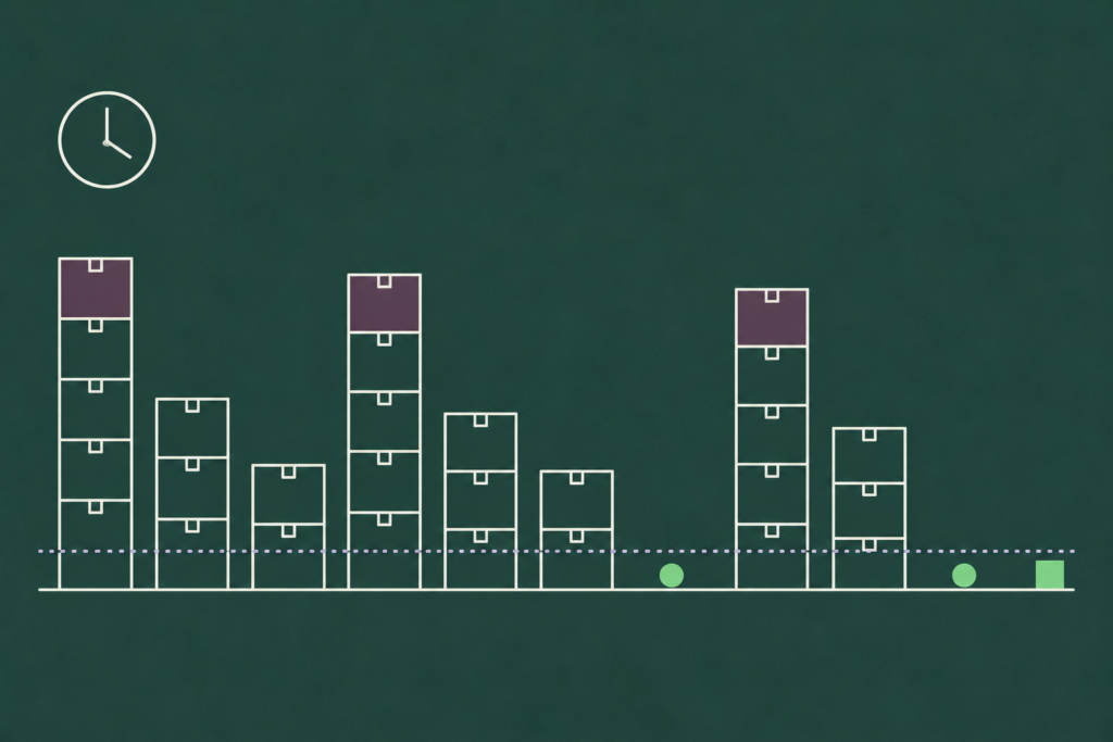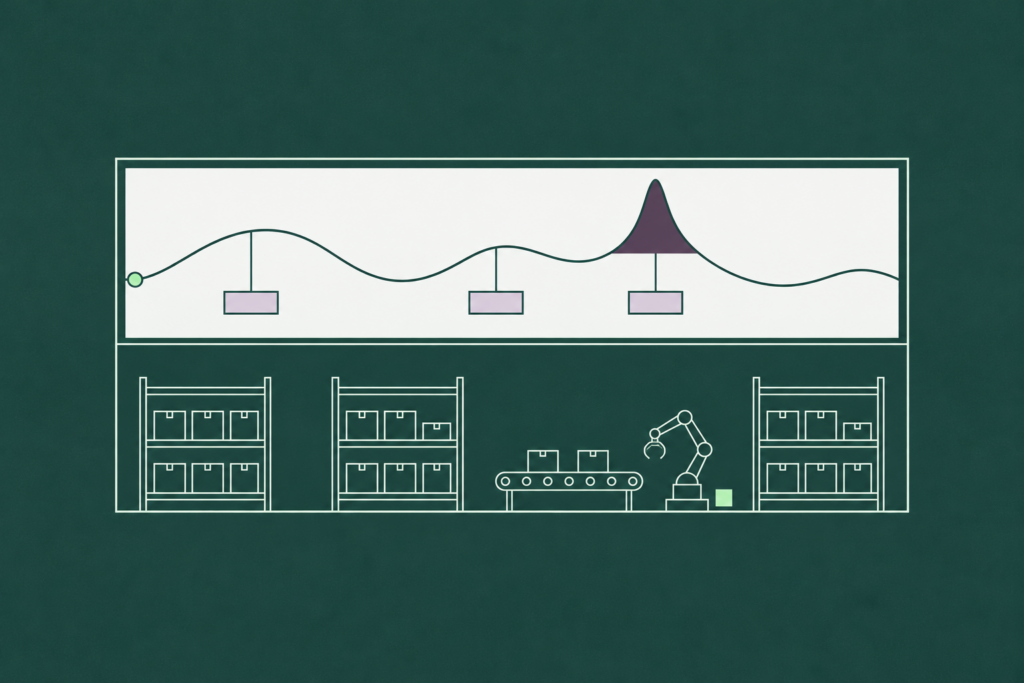
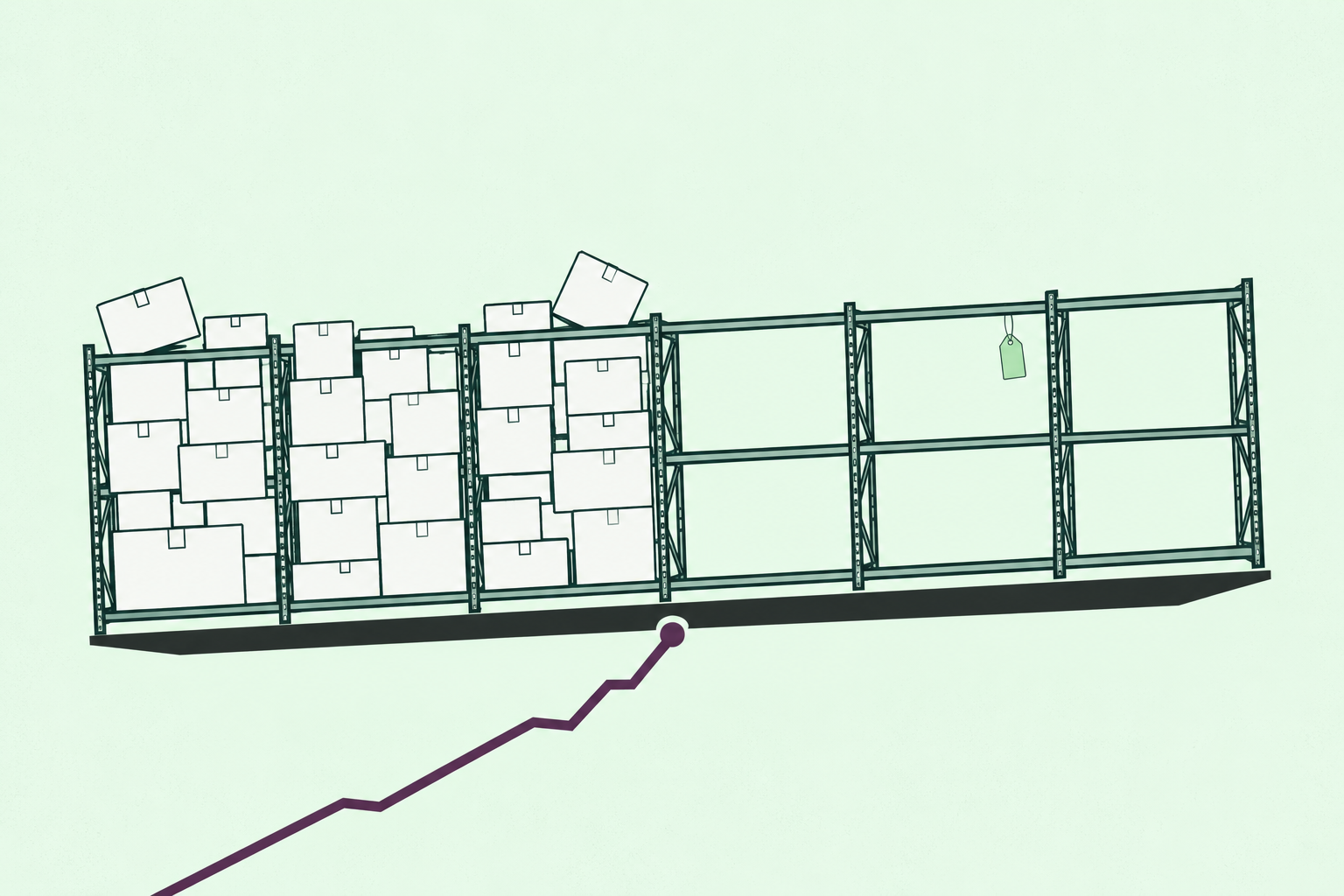
Most inventory problems are forecast problems wearing a disguise.
The excess stock sitting in the distribution center was purchased against a demand number that never materialized. The stockout on the best seller happened because the plan under-called a demand shift the data had been signaling for weeks. Both show up on inventory reports, both get assigned to inventory teams, and both started upstream, in the forecast. Organizations that treat inventory optimization as a warehousing and purchasing discipline keep buying software to manage symptoms. The cause sits one system earlier. The clearest proof is a pattern we see constantly in planning organizations: a company carrying too much of some SKUs and running out of others in the same week, for the same reason.
This article makes that argument concretely: the cost of getting it wrong, what excess inventory and stockouts each cost on their own, the seven levers available to move inventory performance, and the case for treating forecast accuracy as the lever that moves all the others.
What is inventory optimization?
Inventory optimization is the practice of holding the least inventory that still meets target service levels, by balancing the cost of carrying stock against the cost of running out. It covers safety stock, order quantities, replenishment timing and service targets by SKU, and every one of those decisions rests on a demand forecast.
The definition contains a discipline many programs skip: optimization means balancing two costs, and both need to be priced. Which brings us to the table most inventory business cases never build.
The real cost of getting it wrong
Forecast error is expensive in both directions, and asymmetrically so. The table below prices each direction per $1 million of inventory value. Assumptions are stated below the table; adjust them to your own cost structure.
| Error direction | Cost mechanism | Annual cost per $1M of inventory affected |
| Over-forecasting (excess stock) | Carrying cost: capital, warehousing, insurance, shrinkage, obsolescence | $200,000 to $300,000, using the standard published carrying cost range of 20% to 30% of inventory value per year |
| Over-forecasting (obsolete stock) | Write-downs and disposal at end of life; concentrated in short-lifecycle and perishable categories | Additional to carrying cost; realized as margin loss at write-off |
| Under-forecasting (stockouts) | Lost sales at full gross margin, substitution to competitors, contractual service penalties in B2B | Scales with margin and repeat-purchase risk rather than inventory value; a $1M revenue shortfall at 40% margin is $400,000 of gross profit foregone |
| Under-forecasting (recovery) | Expediting: premium freight, overtime, broken production schedules to chase demand already lost | Premium logistics typically costs a multiple of standard freight; recovery spend follows the stockout it failed to prevent |
Assumptions: carrying cost of 20% to 30% annually is the range consistently published across supply chain references (capital cost, storage, handling, insurance, shrinkage and obsolescence combined). Stockout costs are situational and should be modeled from your own margin and customer-switching behavior.
The asymmetry is the important reading. Excess stock bleeds predictably at 20% to 30% a year. Stockouts spike unpredictably and take customer relationships with them. Buffering everything protects against the second cost by maximizing the first, which is precisely the trade a better forecast lets you stop making.
The table makes the two costs look like alternatives, as if a company picks which one to pay. In practice most planning organizations pay both at once. A company can be overstocked and stocking out in the same week, on different SKUs, in the same distribution center: the slow movers bought against last year’s optimism sit in the back while the item that started trending in March is on backorder. Both problems show up on the inventory report. Both get assigned to the inventory team. And both started in the forecast, well before anyone cut a purchase order, because a forecast that over-calls some items and under-calls others produces exactly this shape of pain. Buying more of everything does nothing for it. It just makes the left side of the warehouse heavier.
The reverse is also true, and it’s measurable. In our 2026 accuracy report, a global fast fashion retailer forecasting more than 10,000 SKUs across nearly 5,000 stores saw both halves move in the same deployment. Better forecasts cut overstock by up to 50% and lifted sales 10% to 25%. The sales lift came from fewer stockouts, and the excess reduction came from the same forecast, at the same time. We report those inventory outcomes as observed rather than attributing them to accuracy alone, since reorder policy and planner behavior decide how much of a better forecast reaches the shelf, and what a better forecast is worth downstream sets out that boundary before it gives the numbers.

Excess inventory: what it costs and where it comes from
Excess inventory is stock on hand beyond what you’ll sell before the next replenishment arrives, plus the safety stock you’ve chosen to hold. Everything above that line is excess, whether it’s a pallet of a discontinued flavor or an extra two weeks of a healthy seller. Overstock is the same thing under a warehouse manager’s name for it.
The simple form of the excess inventory formula:
Excess inventory = On-hand stock − (Forecast demand through the next receipt + Safety stock)
Run it per SKU-location, and the result is a list, not a total. That matters, because excess concentrates. In most portfolios we look at, a small share of SKUs holds most of the excess value, and those SKUs are rarely the ones the warehouse team would have guessed.
Where it comes from is more predictable than where it sits. Persistent positive forecast bias is the largest source, because a forecast that runs 5% high on a category builds 5% too much stock every cycle until someone notices the turns falling. Launch optimism is the second: new products get stocked to the sales plan rather than to a demand estimate, and the gap becomes obsolete inventory eighteen months later. Batching against a stale forecast is the third, since an economic order quantity computed when the item sold 400 a week keeps ordering in 400-a-week lots after it drops to 250. Safety stock parameters set once and never recalculated make up the fourth. Discontinuations that nobody plans for strand the rest.
Notice what every item on that list has in common. Each one is a purchase decision that was right about a forecast that turned out to be wrong. The deployment-by-deployment results in our accuracy report show how far the incumbent forecasts were off in each case, and the excess those companies had been carrying was the physical record of that gap.

Inventory carrying cost
Inventory carrying cost is the total annual cost of holding a dollar of inventory, expressed as a percentage of inventory value. The published range is 20% to 30% a year, and it’s higher than most operators assume because storage, the part everyone counts, is usually the smallest component.
Four components make up the figure. Capital cost is the largest: the return the cash tied up in stock would have earned elsewhere, or the interest paid to fund it. Storage and handling cover the warehouse space, labor, equipment and utilities the stock occupies. Service costs include insurance and, in some jurisdictions, inventory taxes. Risk costs cover obsolescence, shrinkage, damage and the markdowns needed to clear stock that aged past its window, and this last component is where short-lifecycle and perishable categories push the total toward the top of the range or past it.
Put it on the excess line from above and the arithmetic is uncomfortable. One million dollars of excess inventory at a 25% carrying cost is $250,000 a year for as long as it sits, before the write-down when it’s finally cleared. A planning team that reduces excess by a third has found $80,000 a year per million without touching service levels, and the reduction usually starts with the forecast bias that created the excess in the first place.

The cost of a stockout
A stockout has a visible cost and an invisible one, and the invisible one is larger.
The visible cost is the sale you didn’t make, valued at full gross margin, plus whatever you spent trying to recover it: premium freight, overtime, a broken production schedule to chase demand that had already left. In B2B the visible cost also includes contractual service penalties and the fill-rate chargebacks that large retail customers apply automatically. All of these are countable, which is why they’re the ones that make it into the business case.
The invisible cost is substitution that becomes permanent. A shopper who couldn’t find your product bought a competitor’s, and some share of them never came back. A retailer that saw two stockouts in a quarter gave the facing to a brand that ships. A B2B account that had to source elsewhere in an emergency now has a second approved supplier it didn’t have before. None of this shows on the inventory report, and all of it compounds, which is why stockouts on a company’s highest-velocity items are so much more expensive than a lost-margin calculation suggests.
Our accuracy report includes one case that puts a figure on it. A steel manufacturer recovered $4M to $5M in annual sales at a single site, revenue that had been lost to stockouts before the deployment, once its forecast stopped under-calling demand on the products that mattered. That’s one site. The figure is reported as observed, and it’s the kind of number that turns a stockout from a service metric into a line the CFO reads.
The practical consequence is a rule most inventory programs get backwards. Stockout cost should set your service level targets by segment, and forecast accuracy should then decide how much stock it takes to hit them. Setting the target first and buffering blindly protects against the visible cost by maximizing the carrying cost from the section above.

The 7 levers of inventory optimization
Seven levers move inventory performance. Each has a primary metric it improves, and one of them moves all the rest.
| Lever | What it changes | Primary metric moved |
| Forecast accuracy | The demand signal every other lever calibrates against | All of the below |
| Safety stock policy | Buffer sizing by measured variability and target service | Working capital, service level |
| Lead times | The exposure window variability acts over | Safety stock requirement, responsiveness |
| SKU segmentation | Differentiated policies by value, velocity, variability | Planning effort allocation, portfolio service |
| Order quantities | Batch sizes balancing ordering cost against holding cost | Cycle stock, inventory turns |
| Phase-in / phase-out | Stock positions through launches and end-of-life | Obsolescence write-offs |
| Service level targets | The protection each segment is entitled to | Inventory-to-service trade-off |
Safety stock policy
Statistical buffers sized from measured demand and lead time variability, per SKU, per service target, using the safety stock formula that fits each segment’s demand pattern. The most common failure is parameters set once and never recalculated, so buffers reflect the variability of two years ago.
Lead times
Shorter and more reliable lead times shrink the window variability operates over, cutting the buffer required at any service level. Lead time reliability is frequently worth more than lead time reduction.
SKU segmentation
An ABC-XYZ grid (value crossed with variability) tells you where precision pays. High-value volatile items justify daily attention; long-tail stable items justify automation. Undifferentiated policies overprotect half the portfolio and underprotect the other half. The fastest way to see whether your segmentation is working is to measure it with the inventory turnover ratio by segment, since undifferentiated policies show up as high turns on the items that needed protection and low turns on the items that didn’t.
Order quantities
Larger batches lower ordering and changeover costs while raising average inventory. The economics move whenever demand shifts, so quantities calibrated to an old forecast quietly become wrong.
Phase-in / phase-out
Launches over-stock on optimism; discontinuations strand inventory that outlives the product. Both are forecasting problems with inventory consequences, and both concentrate obsolescence cost into short windows.
Service level targets
Not every SKU deserves 99%. Setting targets by segment, then letting the safety stock math follow, is how mature operations release working capital without visible service loss.
Why forecast accuracy is the master lever
Work through the list again and notice the dependency. Safety stock formulas take demand variability as an input, and measured against your plan, that variability is forecast error. Segmentation classifies items partly by how predictable they are. Order quantities are computed against expected demand. Phase-in and phase-out are forecasts by definition. Even service level economics shift, because a more accurate forecast delivers any given service target with less stock.
Improve demand forecasting accuracy, and every one of those calculations improves at its next refresh, without any process change in the inventory function itself. The reverse fails: a company can execute six levers flawlessly against a biased forecast and still hold the wrong inventory, positioned confidently in the wrong places. That’s the practical meaning of the disguise argument this article opened with. Fixing the forecast is upstream maintenance; everything downstream inherits it.
The relationship is also quantifiable, which makes it unusual among supply chain investments: cut the standard deviation of forecast error by 30% and statistical safety stock on demand-driven SKUs falls by the same 30%, at identical service. Few initiatives convert into working capital that directly.
That claim needs evidence, and until this year we mostly argued it from the math. Our 2026 accuracy report benchmarks 15 demand forecasting deployments measured against the forecast they already ran, in each company’s own metric, and the AI forecast produced less error than the incumbent in every one. Forecast error fell by 32% on average across 15 demand forecasting deployments. Plug a reduction of that size into the safety stock relationship above and the working capital consequence writes itself, which is why the first step in any inventory program should be to measure forecast accuracy properly, at SKU level, in a metric your finance team accepts, before spending on anything downstream.

Demand variability: measure it before you buffer it
One distinction protects an optimization program from solving the wrong problem: demand variability and demand unpredictability are different quantities. A seasonal product swings widely and predictably; a flat product can drift in ways no one calls. Buffers should be sized against unpredictability, meaning the variability that remains after a competent forecast has explained everything explainable.
The practical test: measure the standard deviation of forecast error, per SKU, rather than the standard deviation of raw demand. Where the two diverge sharply, your current forecast is leaving predictable structure on the table, and inventory is paying for it. That measurement, run across a portfolio, is the fastest diagnostic for whether your next dollar belongs in inventory software or forecasting capability.
Inventory optimization techniques that scale
Two techniques matter most as networks grow. Multi-echelon inventory optimization (MEIO) positions buffers across the network as a system rather than optimizing each location in isolation, recognizing that upstream stock can protect many downstream nodes at once. And policy automation, recalculating safety stocks, reorder points and order quantities on a schedule as demand patterns shift, keeps thousands of SKU-location parameters current where manual review covers dozens.
Both techniques share the same dependency as everything else in this article: they optimize against a demand signal, and they scale the consequences of that signal’s quality, in either direction.
From forecast to fewer stockouts
The operating model that follows from this argument is simple. Generate accurate, machine-learned baseline forecasts at the SKU level. Measure the error that remains. Size buffers against that error rather than against raw history, and recalculate as accuracy improves.
The results at that first step are established: AI/ML forecasting outperforms legacy methods on the error metrics that feed directly into inventory math, and the customer evidence is concrete. Kenvue reduced forecast error (MAPE) by 37% by combining its planners with AI-generated baselines, an improvement its own case study ties to dramatic reductions in both excess stock and shortages, the two failure modes this article has been pricing. One global food and consumer packaged goods manufacturer improved forecast accuracy by 10% to 30% across major product categories while planning thousands of SKUs across its distribution network. And a large, publicly traded automotive aftermarket manufacturer managing more than 100,000 SKUs cut manual data cleansing by roughly 70%, freeing planner capacity for exactly the exception work that inventory precision requires.
If your inventory program has plateaued, price the forecast error it’s absorbing before adding another downstream tool; our guide to supply chain forecasting tools maps the category. To quantify what a stronger baseline would release from your own working capital, request a demo of DemandForecast.ai.