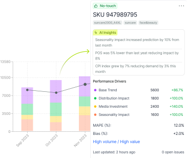
One accuracy number can hide three different problems.
Most accuracy reviews spend their time debating a single percentage. Is 85% good? Is 92% achievable? The debate is misplaced, because the same forecast, scored on the same weeks of the same SKU, can come out at 84.8% accurate or 94.2% accurate depending on which metric you compute. Neither number is wrong. Each one answers a different question, and the real work of measurement is knowing which question your business needs answered.
This guide runs one 12-week dataset for a single SKU through MAPE, WMAPE, bias and forecast value added (FVA), so you can see how each metric reads the identical numbers differently. If you’re newer to the discipline, our guide to demand forecasting covers the fundamentals that sit underneath everything here.
What is forecast accuracy?
Forecast accuracy is the degree to which a demand forecast matches actual observed demand, expressed as a percentage or as an error metric. It’s calculated by comparing forecasted values against actuals over a defined period, at a defined level of granularity (SKU, category, region), using a chosen error measure such as MAPE or WMAPE.
Two details in that definition carry most of the weight. Granularity first: a forecast can be 95% accurate at the national level and 60% accurate at the SKU-store level, and the SKU-store number is the one your replenishment system runs on. Then the choice of measure, which is the subject of the rest of this article.
The forecast accuracy formula
The most common forecast accuracy formula is:
Forecast accuracy = 1 − (|Actual − Forecast| ÷ Actual)
Expressed as a percentage, a week where you forecast 1,000 units and sell 950 scores 1 − (50 ÷ 950) = 94.7% accurate. Across multiple periods, you average the error term first, then subtract from 1. Accuracy is simply the mirror image of error: accuracy = 1 − error. A forecast with 6% WMAPE is 94% accurate on a weighted basis.
Three decisions shape the result before any math happens: the granularity you score at, the lag you score against (the forecast made 4 weeks out, or the one made 1 week out), and the error metric itself. Fix all three in a documented standard, or every accuracy conversation in your business will quietly compare different numbers.
The worked dataset
Every metric below is computed on this same 12 weeks of history for one SKU. Weeks 6 and 10 are post-promotion troughs, which is exactly the kind of irregular demand that separates the metrics from each other.
| Week | Actual | Forecast | Abs. error | Error % of actual |
| 1 | 950 | 1,000 | 50 | 5.3% |
| 2 | 1,010 | 1,000 | 10 | 1.0% |
| 3 | 980 | 1,000 | 20 | 2.0% |
| 4 | 1,040 | 1,000 | 40 | 3.8% |
| 5 | 990 | 1,000 | 10 | 1.0% |
| 6 | 210 | 400 | 190 | 90.5% |
| 7 | 1,020 | 1,000 | 20 | 2.0% |
| 8 | 970 | 1,000 | 30 | 3.1% |
| 9 | 1,000 | 1,000 | 0 | 0.0% |
| 10 | 240 | 400 | 160 | 66.7% |
| 11 | 1,030 | 1,000 | 30 | 2.9% |
| 12 | 960 | 1,000 | 40 | 4.2% |
| Total | 10,400 | 10,800 | 600 |
MAPE: the standard that misleads
MAPE (mean absolute percentage error) averages the weekly percentage errors:
MAPE = average of (|Actual − Forecast| ÷ Actual)
On the dataset: the twelve weekly error percentages average to 15.2% MAPE, or 84.8% accuracy. That looks like a forecast in trouble.
Look at where the error lives, though. Ten of the twelve weeks run between 0% and 5.3% error. The two trough weeks contribute 90.5% and 66.7%, and because MAPE gives every week an equal vote, those two low-volume weeks drag the whole average down. In week 6 the forecast missed by 190 units on 210 units of actual demand. The percentage is enormous; the unit impact is modest.
This is the low-volume distortion problem, and it gets worse as you score at finer granularity, where small denominators are everywhere. A planner managing thousands of SKUs will see MAPE punish the slow movers hardest, even when the units at stake are trivial. MAPE also breaks entirely on zero-demand periods, since you cannot divide by zero.
MAPE remains useful for one thing: comparing forecast quality on a single, reasonably stable series over time. As a portfolio metric, it misleads.
WMAPE: why planners weight it
WMAPE (weighted MAPE) fixes the equal-vote problem by pooling the errors before dividing:
WMAPE = sum of absolute errors ÷ sum of actuals
On the dataset: 600 units of total error against 10,400 units of total demand gives 5.8% WMAPE, or 94.2% accuracy.
Same weeks. Same forecast. MAPE said 84.8%; WMAPE says 94.2%. The difference is that WMAPE weights each week by its volume, so the two small trough weeks count for what they are: about 4% of total demand. A 190-unit miss counts as 190 units, whether it happens in a big week or a small one.
That property is why WMAPE is the practitioner’s default for portfolio-level reporting. It answers the question the supply chain actually asks: of all the units we needed to place correctly, what share did we miss? It aggregates cleanly across SKUs, handles intermittent demand without exploding, and ties directly to inventory and service consequences, which are unit-denominated, never percentage-denominated.
Forecast bias: the direction problem
MAPE and WMAPE both take absolute values, which throws away the sign of the error. Bias puts it back:
Bias = (sum of forecasts − sum of actuals) ÷ sum of actuals
On the dataset: the forecast totaled 10,800 units against 10,400 actual, a +3.8% bias. This forecast over-calls demand, consistently.
Bias is the most operationally expensive error type, because it compounds. A forecast that’s 6% wrong but random will over-call some weeks and under-call others, and inventory buffers absorb the noise. A forecast that’s 4% high every single week builds excess stock every single week. Persistent positive bias fills warehouses; persistent negative bias empties shelves. In S&OP environments, bias also tends to be structural rather than statistical: sales teams protect targets, finance anchors to budget, and the forecast inherits the optimism.
Track bias as a signed running measure alongside WMAPE. A forecast can hold steady on WMAPE while drifting on bias, and the drift is the earlier warning. This is also where AI-based approaches have shown measurable impact: published benchmarks on this site put forecast bias reduction from AI at around 20%, precisely because a model has no quarterly target to defend.
Forecast value added: are your overrides helping?
FVA measures whether each step of your forecasting process improves on a naive baseline, usually “next period equals last period.”
FVA = error of the naive forecast − error of the process step being tested
On the dataset, scoring weeks 2 through 12: the naive forecast produces 36.9% WMAPE, because it walks straight into both demand troughs a week late. The statistical forecast produces 5.8%. The statistical step therefore adds 31.1 points of value. It’s earning its keep.
Now test the human layer. Suppose the demand review raises every statistical number by 5%, a common consensus-meeting outcome. The final forecast now scores 9.0% WMAPE. The override step added negative 3.3 points: the touch made the forecast worse, and without FVA you would never know, because 9.0% still looks respectable in isolation.
Run FVA on every stage that touches the number: statistical model, planner adjustment, consensus override, executive override. In many organizations, the honest finding is that one or more stages consistently subtracts value, and removing that touch is the cheapest accuracy improvement available.
Which metric should you use?
No single metric covers every demand pattern. The matrix below is a defensible starting standard.
| Demand pattern | Recommended metric | Why | Trap to avoid |
| High-volume, stable SKUs | WMAPE, with bias tracked alongside | Volume weighting matches business impact | Reporting MAPE and WMAPE interchangeably in the same review |
| Seasonal SKUs | WMAPE at fixed lag, plus bias by season phase | Lag discipline stops in-season revisions from flattering the score | Scoring the 1-week-out forecast when purchasing commits at 12 weeks |
| Intermittent / slow movers | WMAPE pooled across the segment; unit error (MAD) per SKU | Percentage errors are unstable on small denominators | Any per-SKU MAPE target; zeros and near-zeros make it meaningless |
| New products | Bias first; FVA once history allows | Early forecasts are assumption-driven, so direction matters more than precision | Judging launch forecasts on MAPE in the first weeks of noisy actuals |
What is a good forecast accuracy percentage?
Honest ranges, at SKU level, monthly buckets, measured as WMAPE-based accuracy:
- Stable, high-volume consumer staples: 80% to 90% is strong. Above 90% at SKU level is uncommon and usually reflects aggregation.
- Seasonal and promoted categories: 70% to 85%, depending on promotional intensity.
- Intermittent B2B or long-tail SKUs: 50% to 70% can be genuinely good performance.
- New products: wide misses are normal for the first cycles; measure bias and time-to-stabilize instead.
Any vendor or consultant quoting a universal “good” number without stating granularity, lag and metric is quoting a number you cannot use. Real-world anchors help: Nanit, the smart baby technology company, runs its inventory planning on forecasts operating at roughly 80% accuracy, a figure that sits exactly where a well-run consumer hardware operation should. The more productive question is trajectory: is error falling quarter over quarter, and is bias holding near zero?
How AI lifts accuracy
Measurement tells you where the forecast is wrong. Improving it is a different discipline, and it’s where machine learning models separate from statistical baselines: they ingest far more signals (promotions, pricing, seasonality interactions, external drivers) and they recalibrate continuously instead of waiting for a planner to notice drift. Our overview of AI and machine learning forecasting covers how these models work in production planning environments.
The results are measurable with exactly the metrics in this article. Kenvue reduced forecast error (MAPE) by 37% by combining its planning teams with AI-generated baseline forecasts, an improvement scored on the same error framework its planners already reported against. One global food and consumer packaged goods manufacturer, forecasting across thousands of SKUs, customers and distribution centers, improved forecast accuracy by 10% to 30% across its major product categories. Across deployments, benchmarks published on this site show AI forecasting improving accuracy by 15% to 30% and reducing forecast bias by roughly 20%.
If your accuracy reviews keep producing the same numbers and the same arguments, the constraint is probably the baseline forecast rather than the review process. Evaluating demand forecasting software against your own data, scored with WMAPE, bias and FVA at your operating granularity, is the fastest way to find out. Request a demo to run that evaluation with DemandForecast.ai.